


1、 多重共线性的定义:
多重共线性(Multicollinearity)是指线性回归模型中的解释变量之间由于存在精确相关关系或高度相关。
2、 多重共线性对线性回归模型的影响:
(1) 是否会影响模型的泛化能力?
好多文章中说这个会影响模型的泛化能力,这个不能一概而论,当损失函数最终收敛的情况下,是不影响模型泛化能力的,但是现实中的特征数据是存在噪声的,因此强相关的特征同时使用的话会增加模型受噪声影响的程度,比如X1、X2、X3三个强相关的特征,每个特征受到噪声干扰的程度是0.02,那么用其中一个特征模型受噪声影响的概率为0.02,但如果三个同时使用的话,模型受噪声干扰的程度是1-0.98*0.98*0,98=0.058808,显然比只用一个特征受噪声干扰的程度要大。实际上这增加了模型不稳定的程度,可能会影响模型的泛化能力。
(2) 是否会影响变量的分析?
这个答案是肯定的, 假设有三个特征变量X1, X2, X3其中X2= 2X1,即X1与X2存在共线性关系,如果选取X1,X3, Y = W1*X1 + W3 * X3,假设训练完后回归方程是:Y = 24X1 + 6X3,如果X1、X2、X3同时入模的话,Y = W1*X1 + W2*X2 +W3*X3 =
W1*X1 + W2*2*X1 + W3*X3 = (W1 +2*W2)X1 +W3*X3,另W4=W1 +2*W2则Y=W4*X1 +W3*X3,实际上 Y=W4*X1 +W3*X3 与 Y = W1*X1 + W3 * X3是等价的,则最终模型也应该是Y = 24*X1 + 6*X3,所以 W4=24=W1 + 2*W2,这样W1 和W2就有无穷多组解,比如 (0,24)、(-1, 25), (11, 13)等,会导致模型系数的值不稳定,甚至出现0和负数的情况,这样就没有通过系数值来判断特征的重要性了,无法解释单个变量对模型的影响,当然这是再简化后的理想情况下W3是不变化的假设下,即使W3变化了,W4与W2和W1也保持一种关系,W2与W1的解也是有多解。
(3) 共线性变量的系数是否会对非共线性变量的系数产生影响?
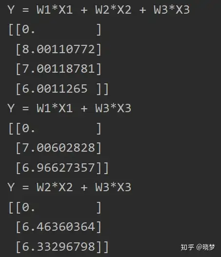
通过实验看是有影响的。假设有一种场景有三个变量x1,x2,x3三个特征变量,y与x1, x2, x3的关系为y = 8 * x1 + 7 * x2 + 6 * x1, 且 x1与x2之间存在共线性,x2 = 2 * x1通过建立简单的线性模型可以看出:再x1,x2,x3同时加入模型和x1、x3加入模型,x2、x3加入模型三种情况下下,x3的系数是变化的:
import numpy as np
from random import sample

def add_random(x, sd):
    '''
    给特征变量随机添加噪音
:param x:
:param sd:
:return:
    '''
num = len(x[0])
    x_new = x + np.random.normal(loc=0, scale=sd, size=num)
    num1 = int(num *0.2)
    data = [i for i in range(0, num)]
    index = sample(data, num1)
    x_new[0][index] = x_new[0][index] + np.random.normal(loc=0, scale=sd * 1.6, size=num1)
    num2 = int(num * 0.16)
    index2 = sample(data, num2)
    x_new[0][index2] = x_new[0][index2] + np.random.normal(loc=0, scale=sd * 1.8, size=num2)
    return x_new


def return_Y_estimate(theta_now, data_x):
    '''
    根据当前的theta求Y的估计值
    传入的data_x的最左侧列为全1,即设X_0 = 1
:param theta_now:
:param data_x:
:return:
    '''
# 确保theta_now为列向量
    theta_now = theta_now.reshape(-1, 1)
    Y_estimate = np.dot(data_x, theta_now)
    return Y_estimate


def return_dJ(theta_now, data_x, y_true):
    '''
    求当前theta的梯度
    传入的data_x的最左侧列为全1,即设X_0 = 1
:param theta_now:
:param data_x:
:param y_true:
:return:
    '''
y_estimate = return_Y_estimate(theta_now, data_x)
    # 共有_N组数据
    N = data_x.shape[0]
    # 求解的theta个数
    num_of_features = data_x.shape[1]
    # 构建
    dJ = np.zeros([num_of_features, 1])

    for i in range(num_of_features):
        dJ[i, 0] = 2 * np.dot((y_estimate - y_true).T, data_x[:, i]) / N

    return dJ


def return_J(theta_now, data_x, y_true):
    '''
    计算J的值
    传入的data_x的最左侧列为全1,即设X_0 = 1
:param theta_now:
:param data_x:
:param y_true:
:return:
    '''
# 共有N组数据
    N = data_x.shape[0]
    temp = y_true - np.dot(data_x, theta_now)
    J = np.dot(temp.T, temp) / N

    return J


def gradient_descent(data_x, data_y, Learning_rate=0.01, ER=1e-10, MAX_LOOP=1e5):
    '''
    梯度下降法求解线性回归
    data_x的一行为一组数据
    data_y为列向量,每一行对应data_x一行的计算结果
    学习率默认为0.3
    误差默认为1e-8
    默认最大迭代次数为1e4
:param data_x:
:param data_y:
:param Learning_rate:
:param ER:
:param MAX_LOOP:
:return:
    '''
# 样本个数为
    num_of_samples = data_x.shape[0]
    # 在data_x的最左侧拼接全1列
    X_0 = np.zeros([num_of_samples, 1])
    new_x = np.column_stack((X_0, data_x))
    # 确保data_y为列向量
    new_y = data_y.reshape(-1, 1)
    # 求解的未知元个数为
    num_of_features = new_x.shape[1]
    # 初始化theta向量
    theta = np.zeros([num_of_features, 1]) * 0.3
    flag = 0  # 定义跳出标志位
    last_J = 0  # 用来存放上一次的Lose Function的值
    ct = 0  # 用来计算迭代次数
    while flag == 0 and ct < MAX_LOOP:
        last_theta = theta
        # 更新theta
        gradient = return_dJ(theta, new_x, new_y)
        theta = theta - Learning_rate * gradient
        er = abs(return_J(last_theta, new_x, new_y) - return_J(theta, new_x, new_y))
        # 误差达到阀值则刷新跳出标志位
        if er < ER:
            flag = 1
        # 叠加迭代次数
        ct += 1
    return theta


def main():
    # 样本数据生成
    # 生成数据以1元为例,要估计的theta数为2个
    num_of_features = 3
    num_of_samples = 1000
    # 设置噪声系数
    rate = 0.05
    X = []

    # for i in range(num_of_features):
    #     X.append(np.random.random([1, num_of_samples]) * 10)
    X.append(np.random.normal(loc=1.6, scale=2, size=num_of_samples).reshape(1,num_of_samples))
    X.append(np.random.normal(loc=1.6, scale=2, size=num_of_samples).reshape(1,num_of_samples))
    X.append(np.random.normal(loc=8, scale=5, size=num_of_samples).reshape(1,num_of_samples))
    print(X[0].shape)
    X1 = X[0]
    X2 = X[0] * 2  #X2 = 2 * X1
    X3 = X[2]
    X1 = add_random(X1, sd=0.001)
    X2 = add_random(X2, sd=0.001)
    X3 = add_random(X3, sd=0.001)
    X_new= []
    X_new.append(X1)
    X_new.append(X2)
    X_new.append(X3)
    X_new = np.array(X_new).reshape(num_of_samples, num_of_features)
    print("X的数据规模为 : ", X_new.shape)
    #X = np.array(X).reshape(num_of_samples, num_of_features)
    # 利用方程生成X对应的Y
    Y = []

    for i in range(num_of_samples):
        Y.append(0 + 8 * X_new[i][0] + 7 * X_new[i][1] + 6 * X_new[i][2] + np.random.rand() * rate)
        #Y.append(0 + 8 * X_new[i][0] + 6 * X_new[i][2] + np.random.rand() * rate)
    Y = np.array(Y).reshape(-1, 1)
    print("Y的数据规模为 : ", Y.shape)

    # 计算并打印结果
    #Y = W1*X1 + W2*X2 + W3*X3
    print('Y = W1*X1 + W2*X2 + W3*X3')
    print(gradient_descent(X_new, Y))

    #Y = W1*X1 + W3*X3
    print('Y = W1*X1 + W3*X3')
    X_new = []
    X_new.append(X1)
    X_new.append(X3)
    num_of_features = 2
    X_new = np.array(X_new).reshape(num_of_samples, num_of_features)
    print(gradient_descent(X_new, Y))

    # Y = W2*X2 + W3*X3
    print('Y = W2*X2 + W3*X3')
    X_new = []
    X_new.append(X2)
    X_new.append(X3)
    num_of_features = 2
    X_new = np.array(X_new).reshape(num_of_samples, num_of_features)
    print(gradient_descent(X_new, Y))

    # Y = W2*X2 + W3*X3
    # print('Y = W3*X3 + W4*X4')
    # X_new = []
    # X4 = X1 + X2
    # X_new.append(X3)
    # X_new.append(X4)
    # num_of_features = 2
    # X_new = np.array(X_new).reshape(num_of_samples, num_of_features)
    # print(gradient_descent(X_new, Y))


if __name__ == '__main__':
    main()
运行结果如下:
3、 对共线性变量的处理
(1)删除共线变量
在风控的评分卡模型中,一般的思想是去掉多重共线性变量,理由是增加模型稳定性,但是相对模型的预测能力来说真的是去掉了就一定好吗,如果是完全共线性的当然是需要删除的,但现实中其实特征变量之间并不是完全共线性的,所以删除有可能会导致预测的信息源减少而导致预测能力下降,其实删除只是一种处理方,当比如 A、B两个特征共线性,那么到底选择删除哪一个也有一些方法,比如通过启发式逐个把特征加入模型看模型效果。
(2)加正则项
前面说在理想情况下没有噪声的情况下,共线性并不会导致泛化能力下降,甚至保留可能会有利于模型的预测能力,但现实中特征变量噪声是存在的,那么减少特征数据的噪声也是处理共线性的一种方法。其实L2正则的本质就是处理特征的噪声问题,因此正则项也是处理共线性的一种方法。
